8.1 Philosophy of Adjustments

- Adjustments for Single Options refer to the strategic modifications traders make to their individual options positions to optimize profitability, manage risk, or adapt to changing market conditions. Unlike multi-leg strategies, single options involve holding either a long call, long put, short call, or short put position. However, market volatility, time decay, and unexpected price movements can make it necessary to adjust these positions rather than simply holding them until expiration.
- The philosophy behind adjusting single options is rooted in flexibility and risk management. Traders aim to either improve their profit potential or mitigate losses by making timely adjustments such as rolling to a new strike price, extending expiration, converting positions into spreads, or hedging with other instruments. Each type of adjustment serves a unique purpose—whether it’s locking in profits, reducing cost basis, or protecting against unfavourable price movements.
- Successful adjustments require careful analysis of factors like implied volatility, time decay (theta), and underlying asset trends. By proactively adjusting options positions, traders can adapt to evolving market conditions while maintaining control over risk exposure.
- The philosophy of adjustments in options trading revolves around the principle that markets are dynamic, and positions should evolve accordingly. Adjustments are made to optimize performance, manage risk, and adapt to changing conditions.
-
Why Adjust?
The core philosophy behind adjusting options positions stems from the idea that traders should actively manage their trades rather than passively hoping for favourable outcomes. Adjustments help:
- Protect Capital– Limiting losses when a trade moves against expectations.
- Maximize Profits– Locking in gains or repositioning to capitalize on new trends.
- Adapt to Volatility– Responding to market fluctuations instead of being caught off guard.
-
The Balance Between Risk and Reward
Every adjustment has trade-offs. For example:
- Adding hedges may reduce risk, but it could also limit potential upside.
- Rolling a position may extend timefor an expected move, but it could increase cost. Understanding these trade-offs allows traders to adjust strategically rather than react emotionally.
-
Active vs. Passive Management
A passive trader might hold onto an option until expiration, accepting whatever outcome unfolds. An active trader, however, continually monitors and makes strategic adjustments, such as:
- Rolling to a new strike price or expiration date.
- Hedging with other options or assets.
- Scaling in or out of positions based on market sentiment.
-
Factors Influencing Adjustments
The philosophy of adjustments considers several key factors:
- Market Trend– If the overall market direction changes, adjustments may be necessary.
- Volatility– High volatility can lead to sudden shifts, prompting proactive risk management.
- Time Decay– Options lose value as expiration approaches, requiring timely action.
- Liquidity– Ensuring that adjustments don’t lead to excessive transaction costs or poor execution.
-
Psychological Discipline
Successful traders align adjustments with logic, not emotion. FOMO (fear of missing out) and panic selling often lead to irrational decisions. A structured approach keeps adjustments based on strategy rather than speculation.
Timing Context: When to Adjust?
Timing is crucial for making cost-effective and strategic adjustments. The objective is to protect capital while allowing the trade enough room to play out.
Early Adjustments (e.g., Delta around 0.3–0.5):
These can help reposition before too much adverse movement, but risk acting on short-term volatility.
Optimal Adjustment Windows:
- When Delta approaches or exceeds 0.8, indicating the trade is becoming unbalanced or directional.
- When Days to Expiry (DTE) > 5, allowing time for Theta to contribute positively.
- When Implied Volatility (IV) is high, enabling better credit when adjusting positions.
Key Metrics for Triggering Adjustments
Use objective, pre-defined criteria to avoid emotional adjustments:
- Delta moves beyond a threshold (e.g., ±0.6 to ±0.8)
- Underlying breaches support or resistance levels
- IV crush or spike significantly alters strategy expectations
- Premium decay reaches or exceeds 60%, signaling reduced profit potential or shift in risk-reward
Common Adjustment Mistakes
Understanding and avoiding these common pitfalls can significantly enhance trade outcomes:
- Adjusting too early out of fear, prematurely closing or changing a viable position
- Over-adjusting, resulting in excessive commissions and increased position complexity
- Converting trades into complex spreadswith unfavorable reward-to-risk ratios, which can be harder to manage effectively
8.2 Adjustments for Long Call positions
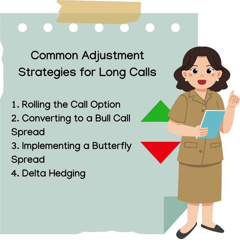
Common Adjustment Strategies for Long Calls
-
Rolling the Call Option
Rolling entails closing an existing option position and opening a new one with different terms.
- Rolling Up: If the underlying asset’s price has increased, you might sell the current call and purchase another with a higher strike price, potentially extending the expiration. This locks in some gains while maintaining a bullish stance.
- Rolling Down: If the asset’s price decreases, selling the current call and buying another with a lower strike price can reduce the breakeven point, albeit with an additional premium cost.
- Rolling Out: Extending the expiration date provides more time for the asset to move favourably, which is beneficial if the current option is nearing expiration without significant movement.
-
Converting to a Bull Call Spread
Transforming a long call into a bull call spread involves selling a call option at a higher strike price while retaining the original long call. This strategy:
- Reduces Net Premium: The premium received from the sold call offsets the cost of the long call.
- Limits Upside Potential: While profits are capped, the strategy mitigates potential losses if the asset doesn’t rise as anticipated.
For instance, if you own a call option with a ₹1,500 strike price on a stock currently trading at ₹1,520, selling a ₹1,550 strike call can create a spread that benefits from moderate price increases.
-
Implementing a Butterfly Spread
A butterfly spread combines multiple options to profit from minimal price movement in the underlying asset. It involves:
- Buying one call at a lower strike price
- Selling two calls at a middle strike price
- Buying one call at a higher strike price
This strategy is suitable when expecting the asset to remain near a specific price, allowing for limited risk and potential profit if the asset’s price stays within a targeted range.
-
Delta Hedging
Delta hedging involves offsetting the directional risk of a position by balancing the delta (rate of change of the option’s price relative to the underlying asset’s price). For a long call:
- If the position has a high positive delta, selling shares of the underlying asset can neutralize the delta, protecting against adverse price movements.
- This approach requires continuous monitoring and adjustment as the delta changes with market movements.
Long Call Adjustments
Long calls offer unlimited upside, but they’re sensitive to time decay (Theta) and volatility changes (Vega). Therefore, managing them through timely adjustments is crucial to optimize returns and control risk.
Adjustment Techniques: Rolling and Converting
Rolling and converting are two primary adjustment tools for long calls:
- Rolling Up: Sell the existing call and buy a higher strike to capture gains and realign the position with the new market direction.
- Rolling Down and Out: Move to a lower strike and a later expiry to reduce cost and buy more time when the market moves against the position.
- Converting to Bull Call Spread: Sell a higher strike against the existing long call to reduce Theta decay and lock in cost, while capping potential profit.
- Closing or Re-structuring: When premiums collapse due to a volatility crash or nearing expiry, it’s often best to exit or restructure.
Situation-Based Adjustment Strategy
|
Situation |
Adjustment |
Objective |
|
Spot rises quickly |
Roll up or sell partial quantity |
Lock in gains |
|
Spot falls below breakeven |
Roll down and out |
Lower cost, extend time |
|
Time decay hitting hard |
Convert to Bull Call Spread |
Reduce Theta drag |
|
Volatility crashes |
Close or convert |
Premiums are dead |
Real Example – Converting to Bull Call Spread
Initial Trade Setup:
Bought Nifty 22,000 CE at ₹100
Market Movement:
Nifty rises to 22,150
The 22,000 CE now trades at ₹140
Implied Volatility drops
Adjustment Strategy:
Sell 22,300 CE at ₹50
New Position:
- Long 22,000 CE at ₹100
- Short 22,300 CE at ₹50
- Net cost = ₹100 – ₹50 = ₹50
- Spread width = 300 points (22,300 – 22,000)
- Maximum profit = ₹300 – ₹50 = ₹250
Why this Works:
- Locks in partial gains from the move up
- Protects against further IV drop or time decay
- Maintains positive reward-to-risk profile
- Limits loss to the ₹50 net debit while capping upside at ₹250 profit
8.3 Adjustments for Short Calls, Long Puts and Short Put positions
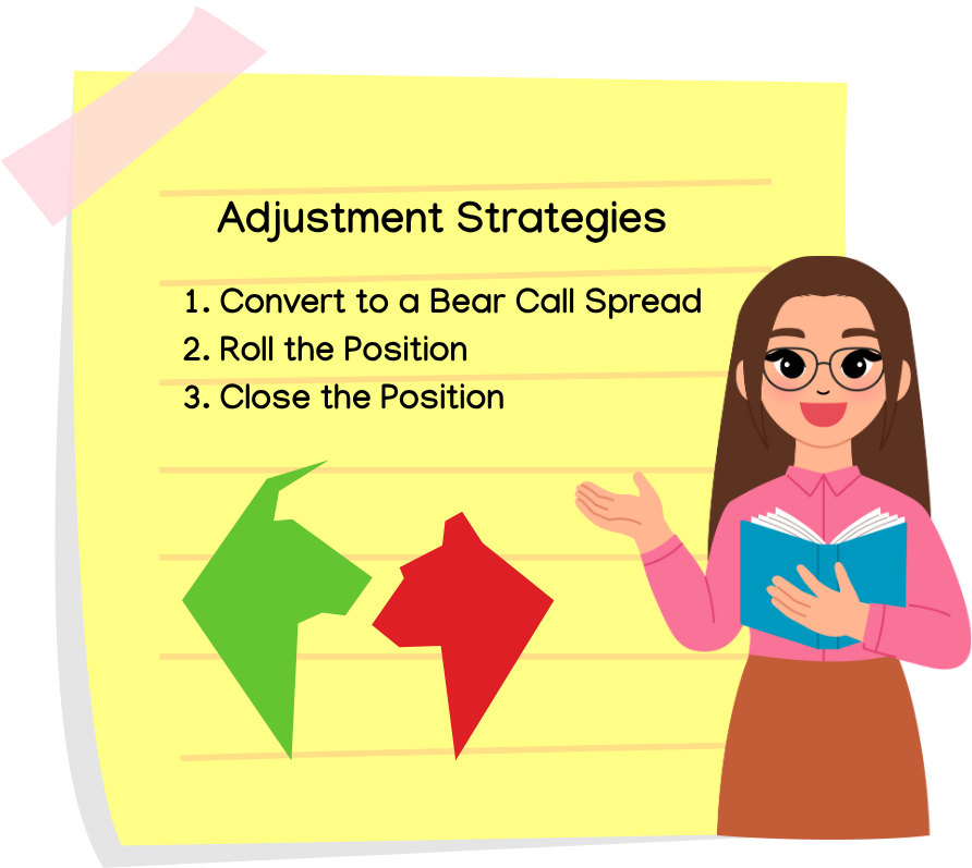
Adjustments for Short Call Positions
A short call involves selling a call option, anticipating that the underlying asset’s price will remain below the strike price. However, if the asset’s price rises significantly, the position can incur substantial losses.
Adjustment Strategies:
- Convert to a Bear Call Spread: Buy a higher strike call option to limit potential losses, transforming the position into a bear call spread.
- Roll the Position: Close the current short call and open a new one with a higher strike price and/or a later expiration date to manage risk and potentially collect additional premium.
- Close the Position: If the outlook changes or risk becomes too high, closing the position can prevent further losses.
Adjustments for Long Put Positions
A long put involves buying a put option, expecting the underlying asset’s price to decline. If the price doesn’t fall as anticipated, the option may lose value.
Adjustment Strategies:
- Roll Down and Out: Sell the current put and buy another with a lower strike price and a later expiration to extend the trade’s duration and adjust to the new market outlook.
- Convert to a Bear Put Spread: Sell a put option at a lower strike price to offset some of the premium paid, reducing the position’s cost basis.
- Close the Position: If the asset’s price is rising or time decay is eroding the option’s value, closing the position can limit losses.
Adjustments for Short Put Positions
A short put involves selling a put option, anticipating that the underlying asset’s price will remain above the strike price. If the price falls below the strike, the position can incur losses.
Adjustment Strategies:
- Convert to a Bull Put Spread: Buy a lower strike put option to limit potential losses, transforming the position into a bull put spread.
- Roll Down and Out: Close the current short put and open a new one with a lower strike price and/or a later expiration to manage risk and potentially collect additional premium.
- Accept Assignment: If willing to own the underlying asset, accept assignment and purchase the stock at the strike price, potentially at a discount if the asset’s price recovers.
Short Call, Long Put, Short Put
This section focuses on tactical management of three commonly used options positions. While each serves a unique strategic purpose, all require timely adjustments and disciplined risk controls.
Short Call – Managing Risk in a Capped Premium Trade
Short calls are used for range-bound or bearish views, but they carry unlimited loss potential if unhedged.
Adjustment Trigger:
- If spot nears the short strike and 80% of premium is already consumed, consider adjusting or closing the position.
Actionable Rule:
- Don’t hold on for the last 20% of premium — the risk-to-reward becomes highly skewed.
Hedging Tip:
- Always hedge with a long call 200–300 points above the short strike.
This converts it into a bear call spread, creating a defined loss structure while still benefiting from time decay.
Long Put – Managing Directional Bearish Bets
Long puts are high-reward bearish trades but are sensitive to Theta and rely on strong directional movement.
When to Convert to Bear Put Spread:
-
- IV is elevated (to gain credit when selling the lower strike)
- Time decay is accelerating
- No sharp fall is expected in the near term
Conversion Strategy:
-
- Sell a lower strike put to form a bear put spread, reducing net cost and limiting downside.
Alternative Strategy – Synthetic Short Straddle:
-
- Sell weekly OTM calls against the long put when expecting consolidation
- This creates a synthetic short straddle or short strangle, generating income while retaining downside exposure.
Use this only when IV is high and movement is expected to be muted in the short term.
Short Put – Managing Risk in Bullish Trades
Short puts are bullish trades that benefit from time decay and rising or sideways markets. However, they carry significant downside risk if the spot falls sharply.
Adjustment Rule:
-
- Do not wait for the put to go deep ITM.
If the spot breaks a major support level, roll early to reduce directional exposure and regain control.
- Do not wait for the put to go deep ITM.
Risk Management Tip – Insurance Put:
Always hedge with a long deep OTM put (500–700 points away) when VIX < 14.
This acts as an insurance policy for a sharp unexpected fall and reduces tail risk
8.4 Trade Management using sophisticated Conditional Order
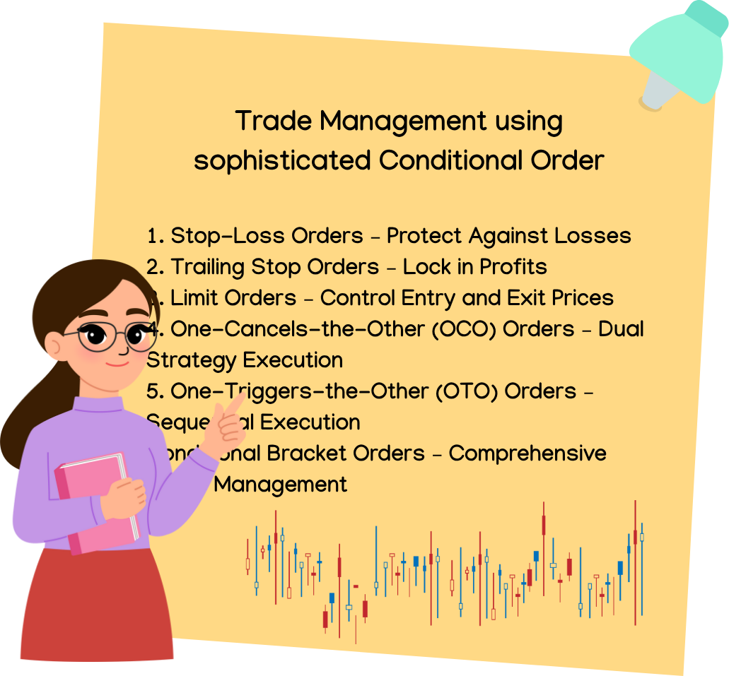
Conditional orders are an essential tool in trading that allow investors to set predefined instructions for trade execution. These orders help traders manage risk, automate decision-making, and ensure more disciplined trading strategies. Below is a detailed explanation of each type of sophisticated conditional order:
-
Stop-Loss Orders – Protect Against Losses
A stop-loss order is designed to limit losses by automatically selling a position when the price drops below a specified level. This prevents further downside exposure and is a key risk management tool for traders.
- How It Works:Traders set a price at which they are willing to exit a trade if the market moves against them. Once the asset price reaches or falls below this level, the order is executed.
- Example:If a trader buys a stock at ₹500, they may set a stop-loss at ₹480. If the stock price drops to ₹480 or lower, the stop-loss order executes automatically, selling the stock and preventing further losses.
-
Trailing Stop Orders – Lock in Profits
A trailing stop order dynamically adjusts the stop price as the asset price moves in a favourable direction. This allows traders to protect profits while staying in the trade as long as the price continues to rise.
- How It Works:Instead of setting a fixed stop price, traders set a trailing amount (in percentage or absolute value). The stop price moves upwards as the stock price increases but remains fixed if the stock starts declining.
- Example:If a trader buys a stock at ₹500 and sets a trailing stop of ₹10, the stop price initially starts at ₹490. If the stock rises to ₹520, the stop price moves to ₹510. If the stock later falls to ₹510 or below, the position is automatically sold.
-
Limit Orders – Control Entry and Exit Prices
A limit order ensures that a trade is executed only at a specific price or better. Traders use these orders to avoid buying or selling at unfavourable market prices.
- How It Works:Traders specify a price at which they are willing to buy or sell an asset. The trade only occurs if the market reaches this price or better.
- Example:A trader wants to buy a stock currently trading at ₹500 but doesn’t want to pay more than ₹495. They place a limit order at ₹495, ensuring that the trade only executes if the price reaches ₹495 or lower.
-
One-Cancels-the-Other (OCO) Orders – Dual Strategy Execution
An OCO order consists of two orders: one aimed at taking profit and the other aimed at limiting losses. If one order executes, the other is automatically cancelled, preventing conflicting trade execution.
- How It Works:Traders set up a take-profit and stop-loss order simultaneously. If the price reaches the profit target, the stop-loss order is cancelled, and vice versa.
- Example:A trader buys a stock at ₹500 and sets a take-profit order at ₹550 and a stop-loss order at ₹480. If the price reaches ₹550, the stock is sold for profit, and the stop-loss order is cancelled.
-
One-Triggers-the-Other (OTO) Orders – Sequential Execution
An OTO order ensures that the execution of a primary order triggers a secondary order. This is useful for structured trade setups.
- How It Works:The initial trade execution activates a follow-up order, ensuring a smooth transition in trade management.
- Example:A trader buys a stock at ₹500. Once this purchase is completed, a stop-loss order at ₹480 is automatically placed. This reduces risk without requiring manual input.
-
Conditional Bracket Orders – Comprehensive Trade Management
Bracket orders allow traders to set an entry price, a take-profit target, and a stop-loss in one command. This is useful for fully automated trade management.
- How It Works:When the entry order executes, bracket conditions automatically apply, ensuring a structured exit plan.
- Example:A trader buys a stock at ₹500, sets a take-profit order at ₹550, and a stop-loss order at ₹480. If the price reaches ₹550, the stock is sold for profit. If it drops to ₹480, the stock is sold to prevent losses.
Risk in High IV Spikes – Be Cautious
- High Implied Volatility (IV)can cause wide bid–ask spreads and sudden price jumps.
- Risk: Multiple conditional orders may trigger simultaneously, leading to over-hedging or duplicate positions.
- Tip: During volatile events (e.g., earnings, Fed events), reduce active OCO/OTO useor lower position sizing.
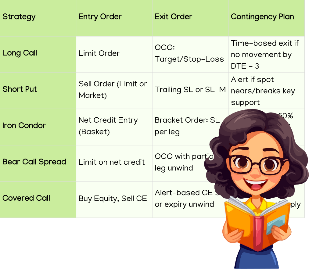
8.5 Strategy-Based Conditional Order Mapping
|
Strategy |
Entry Order |
Exit Order |
Contingency Plan |
|
Long Call |
Limit Order |
OCO: Target/Stop-Loss |
Time-based exit if no movement by DTE – 3 |
|
Short Put |
Sell Order (Limit or Market) |
Trailing SL or SL-M |
Alert if spot nears/breaks key support |
|
Iron Condor |
Net Credit Entry (Basket) |
Bracket Order: SL per leg |
Auto-exit at 50% profit or DTE < 5 days |
|
Bear Call Spread |
Limit on net credit |
OCO with partial leg unwind |
Roll up if IV expands and price moves higher |
|
Covered Call |
Buy Equity, Sell CE |
Alert-based CE SL or expiry unwind |
Adjust strike if stock rises sharply |
8.6 Adjustment ROI Table – Understanding the Value of Adjusting Trades

This table helps quantify how smart adjustments can reduce potential losses, improve risk–reward ratios, and provide flexibility when the market moves against you.
|
Scenario |
Original Trade P&L |
Adjusted Trade P&L |
Benefit |
|
Long Call held to expiry (OTM) |
–₹6,000 |
–₹1,500 (converted to spread) |
75% loss reduction |
|
Short Put without hedge |
–₹18,000 |
–₹5,000 (rolled down + hedged) |
Significant risk reduction + flexibility |
Long Call Held to Expiry vs. Converted to Bull Call Spread
Original Scenario: You buy a Nifty 22,000 CE at ₹120. The market doesn’t move enough, and the option expires out-of-the-money (OTM).
Loss = Total premium paid = –₹6,000
Adjusted Scenario: Midway through the trade, you sell a higher strike CE (e.g., 22,300 CE at ₹70), converting the position into a Bull Call Spread.
- New net debit = ₹120 – ₹70 = ₹50
- Even if the trade doesn’t reach full profit, the sale of the second leg offsets some cost, reducing the total loss.
- Adjusted Loss = –₹1,500 (if spread expires below long strike)
- Benefit: You reduce the loss by 75%, thanks to the time-value salvage and lower Theta drag.
Short Put Without Hedge vs. Rolled Down + Hedged
Original Scenario: You sell a Nifty 22,000 PE for ₹120. Market falls sharply; the spot goes below 21,800.
- The put finishes deep in-the-money, and you’re assigned or face a mark-to-market (MTM) loss.
- Loss = ~₹18,000 (depending on how far spot drops)
Adjusted Scenario:
- When support breaks, you roll the put down to 21,800 and extend expiry (more time).
- Additionally, you buy a deep OTM protective put (e.g., 21,300 PE) as insurance.
- This reduces delta exposure and creates a limited-risk spread.
- Adjusted Loss = –₹5,000 (if market stabilizes or reverses slightly)
- Benefit: You cut risk sharply, stay in the trade longer, and protect against tail risk.
Why This Matters
Adjustments are not just about turning losers into winners.
They’re about reducing damage, regaining control, and positioning smarter when the market changes.
This approach can:
- Improve long-term expectancy
- Reduce emotional stress
- Free up margin or capital earlier
8.7 Adjustment Decision Tree – Flowchart
Key Explanation of Decision Points:
Trade Moving Against You?
- If not, no action is needed.
- If yes, evaluate time and volatility.
Time Remaining > 5 DTE?
- If expiry is near, options lose flexibility.
- If time remains, adjustments are still feasible.
Is IV High?
- High IV allows rolling or converting to spreads for credit.
- Low IV limits premiums — better to cut risk.
Support/Resistance Breached?
- If yes, trend shift is likely. Consider repositioning.
- If no, avoid premature action.
Theta Decay Accelerating?
- If yes, turn long options into spreads or exit.
- If no, observe.
8.1 Philosophy of Adjustments
- Adjustments for Single Options refer to the strategic modifications traders make to their individual options positions to optimize profitability, manage risk, or adapt to changing market conditions. Unlike multi-leg strategies, single options involve holding either a long call, long put, short call, or short put position. However, market volatility, time decay, and unexpected price movements can make it necessary to adjust these positions rather than simply holding them until expiration.
- The philosophy behind adjusting single options is rooted in flexibility and risk management. Traders aim to either improve their profit potential or mitigate losses by making timely adjustments such as rolling to a new strike price, extending expiration, converting positions into spreads, or hedging with other instruments. Each type of adjustment serves a unique purpose—whether it’s locking in profits, reducing cost basis, or protecting against unfavourable price movements.
- Successful adjustments require careful analysis of factors like implied volatility, time decay (theta), and underlying asset trends. By proactively adjusting options positions, traders can adapt to evolving market conditions while maintaining control over risk exposure.
- The philosophy of adjustments in options trading revolves around the principle that markets are dynamic, and positions should evolve accordingly. Adjustments are made to optimize performance, manage risk, and adapt to changing conditions.
-
Why Adjust?
The core philosophy behind adjusting options positions stems from the idea that traders should actively manage their trades rather than passively hoping for favourable outcomes. Adjustments help:
- Protect Capital– Limiting losses when a trade moves against expectations.
- Maximize Profits– Locking in gains or repositioning to capitalize on new trends.
- Adapt to Volatility– Responding to market fluctuations instead of being caught off guard.
-
The Balance Between Risk and Reward
Every adjustment has trade-offs. For example:
- Adding hedges may reduce risk, but it could also limit potential upside.
- Rolling a position may extend timefor an expected move, but it could increase cost. Understanding these trade-offs allows traders to adjust strategically rather than react emotionally.
-
Active vs. Passive Management
A passive trader might hold onto an option until expiration, accepting whatever outcome unfolds. An active trader, however, continually monitors and makes strategic adjustments, such as:
- Rolling to a new strike price or expiration date.
- Hedging with other options or assets.
- Scaling in or out of positions based on market sentiment.
-
Factors Influencing Adjustments
The philosophy of adjustments considers several key factors:
- Market Trend– If the overall market direction changes, adjustments may be necessary.
- Volatility– High volatility can lead to sudden shifts, prompting proactive risk management.
- Time Decay– Options lose value as expiration approaches, requiring timely action.
- Liquidity– Ensuring that adjustments don’t lead to excessive transaction costs or poor execution.
-
Psychological Discipline
Successful traders align adjustments with logic, not emotion. FOMO (fear of missing out) and panic selling often lead to irrational decisions. A structured approach keeps adjustments based on strategy rather than speculation.
Timing Context: When to Adjust?
Timing is crucial for making cost-effective and strategic adjustments. The objective is to protect capital while allowing the trade enough room to play out.
Early Adjustments (e.g., Delta around 0.3–0.5):
These can help reposition before too much adverse movement, but risk acting on short-term volatility.
Optimal Adjustment Windows:
- When Delta approaches or exceeds 0.8, indicating the trade is becoming unbalanced or directional.
- When Days to Expiry (DTE) > 5, allowing time for Theta to contribute positively.
- When Implied Volatility (IV) is high, enabling better credit when adjusting positions.
Key Metrics for Triggering Adjustments
Use objective, pre-defined criteria to avoid emotional adjustments:
- Delta moves beyond a threshold (e.g., ±0.6 to ±0.8)
- Underlying breaches support or resistance levels
- IV crush or spike significantly alters strategy expectations
- Premium decay reaches or exceeds 60%, signaling reduced profit potential or shift in risk-reward
Common Adjustment Mistakes
Understanding and avoiding these common pitfalls can significantly enhance trade outcomes:
- Adjusting too early out of fear, prematurely closing or changing a viable position
- Over-adjusting, resulting in excessive commissions and increased position complexity
- Converting trades into complex spreadswith unfavorable reward-to-risk ratios, which can be harder to manage effectively
8.2 Adjustments for Long Call positions
Common Adjustment Strategies for Long Calls
-
Rolling the Call Option
Rolling entails closing an existing option position and opening a new one with different terms.
- Rolling Up: If the underlying asset’s price has increased, you might sell the current call and purchase another with a higher strike price, potentially extending the expiration. This locks in some gains while maintaining a bullish stance.
- Rolling Down: If the asset’s price decreases, selling the current call and buying another with a lower strike price can reduce the breakeven point, albeit with an additional premium cost.
- Rolling Out: Extending the expiration date provides more time for the asset to move favourably, which is beneficial if the current option is nearing expiration without significant movement.
-
Converting to a Bull Call Spread
Transforming a long call into a bull call spread involves selling a call option at a higher strike price while retaining the original long call. This strategy:
- Reduces Net Premium: The premium received from the sold call offsets the cost of the long call.
- Limits Upside Potential: While profits are capped, the strategy mitigates potential losses if the asset doesn’t rise as anticipated.
For instance, if you own a call option with a ₹1,500 strike price on a stock currently trading at ₹1,520, selling a ₹1,550 strike call can create a spread that benefits from moderate price increases.
-
Implementing a Butterfly Spread
A butterfly spread combines multiple options to profit from minimal price movement in the underlying asset. It involves:
- Buying one call at a lower strike price
- Selling two calls at a middle strike price
- Buying one call at a higher strike price
This strategy is suitable when expecting the asset to remain near a specific price, allowing for limited risk and potential profit if the asset’s price stays within a targeted range.
-
Delta Hedging
Delta hedging involves offsetting the directional risk of a position by balancing the delta (rate of change of the option’s price relative to the underlying asset’s price). For a long call:
- If the position has a high positive delta, selling shares of the underlying asset can neutralize the delta, protecting against adverse price movements.
- This approach requires continuous monitoring and adjustment as the delta changes with market movements.
Long Call Adjustments
Long calls offer unlimited upside, but they’re sensitive to time decay (Theta) and volatility changes (Vega). Therefore, managing them through timely adjustments is crucial to optimize returns and control risk.
Adjustment Techniques: Rolling and Converting
Rolling and converting are two primary adjustment tools for long calls:
- Rolling Up: Sell the existing call and buy a higher strike to capture gains and realign the position with the new market direction.
- Rolling Down and Out: Move to a lower strike and a later expiry to reduce cost and buy more time when the market moves against the position.
- Converting to Bull Call Spread: Sell a higher strike against the existing long call to reduce Theta decay and lock in cost, while capping potential profit.
- Closing or Re-structuring: When premiums collapse due to a volatility crash or nearing expiry, it’s often best to exit or restructure.
Situation-Based Adjustment Strategy
|
Situation |
Adjustment |
Objective |
|
Spot rises quickly |
Roll up or sell partial quantity |
Lock in gains |
|
Spot falls below breakeven |
Roll down and out |
Lower cost, extend time |
|
Time decay hitting hard |
Convert to Bull Call Spread |
Reduce Theta drag |
|
Volatility crashes |
Close or convert |
Premiums are dead |
Real Example – Converting to Bull Call Spread
Initial Trade Setup:
Bought Nifty 22,000 CE at ₹100
Market Movement:
Nifty rises to 22,150
The 22,000 CE now trades at ₹140
Implied Volatility drops
Adjustment Strategy:
Sell 22,300 CE at ₹50
New Position:
- Long 22,000 CE at ₹100
- Short 22,300 CE at ₹50
- Net cost = ₹100 – ₹50 = ₹50
- Spread width = 300 points (22,300 – 22,000)
- Maximum profit = ₹300 – ₹50 = ₹250
Why this Works:
- Locks in partial gains from the move up
- Protects against further IV drop or time decay
- Maintains positive reward-to-risk profile
- Limits loss to the ₹50 net debit while capping upside at ₹250 profit
8.3 Adjustments for Short Calls, Long Puts and Short Put positions
Adjustments for Short Call Positions
A short call involves selling a call option, anticipating that the underlying asset’s price will remain below the strike price. However, if the asset’s price rises significantly, the position can incur substantial losses.
Adjustment Strategies:
- Convert to a Bear Call Spread: Buy a higher strike call option to limit potential losses, transforming the position into a bear call spread.
- Roll the Position: Close the current short call and open a new one with a higher strike price and/or a later expiration date to manage risk and potentially collect additional premium.
- Close the Position: If the outlook changes or risk becomes too high, closing the position can prevent further losses.
Adjustments for Long Put Positions
A long put involves buying a put option, expecting the underlying asset’s price to decline. If the price doesn’t fall as anticipated, the option may lose value.
Adjustment Strategies:
- Roll Down and Out: Sell the current put and buy another with a lower strike price and a later expiration to extend the trade’s duration and adjust to the new market outlook.
- Convert to a Bear Put Spread: Sell a put option at a lower strike price to offset some of the premium paid, reducing the position’s cost basis.
- Close the Position: If the asset’s price is rising or time decay is eroding the option’s value, closing the position can limit losses.
Adjustments for Short Put Positions
A short put involves selling a put option, anticipating that the underlying asset’s price will remain above the strike price. If the price falls below the strike, the position can incur losses.
Adjustment Strategies:
- Convert to a Bull Put Spread: Buy a lower strike put option to limit potential losses, transforming the position into a bull put spread.
- Roll Down and Out: Close the current short put and open a new one with a lower strike price and/or a later expiration to manage risk and potentially collect additional premium.
- Accept Assignment: If willing to own the underlying asset, accept assignment and purchase the stock at the strike price, potentially at a discount if the asset’s price recovers.
Short Call, Long Put, Short Put
This section focuses on tactical management of three commonly used options positions. While each serves a unique strategic purpose, all require timely adjustments and disciplined risk controls.
Short Call – Managing Risk in a Capped Premium Trade
Short calls are used for range-bound or bearish views, but they carry unlimited loss potential if unhedged.
Adjustment Trigger:
- If spot nears the short strike and 80% of premium is already consumed, consider adjusting or closing the position.
Actionable Rule:
- Don’t hold on for the last 20% of premium — the risk-to-reward becomes highly skewed.
Hedging Tip:
- Always hedge with a long call 200–300 points above the short strike.
This converts it into a bear call spread, creating a defined loss structure while still benefiting from time decay.
Long Put – Managing Directional Bearish Bets
Long puts are high-reward bearish trades but are sensitive to Theta and rely on strong directional movement.
When to Convert to Bear Put Spread:
-
- IV is elevated (to gain credit when selling the lower strike)
- Time decay is accelerating
- No sharp fall is expected in the near term
Conversion Strategy:
-
- Sell a lower strike put to form a bear put spread, reducing net cost and limiting downside.
Alternative Strategy – Synthetic Short Straddle:
-
- Sell weekly OTM calls against the long put when expecting consolidation
- This creates a synthetic short straddle or short strangle, generating income while retaining downside exposure.
Use this only when IV is high and movement is expected to be muted in the short term.
Short Put – Managing Risk in Bullish Trades
Short puts are bullish trades that benefit from time decay and rising or sideways markets. However, they carry significant downside risk if the spot falls sharply.
Adjustment Rule:
-
- Do not wait for the put to go deep ITM.
If the spot breaks a major support level, roll early to reduce directional exposure and regain control.
- Do not wait for the put to go deep ITM.
Risk Management Tip – Insurance Put:
Always hedge with a long deep OTM put (500–700 points away) when VIX < 14.
This acts as an insurance policy for a sharp unexpected fall and reduces tail risk
8.4 Trade Management using sophisticated Conditional Order
Conditional orders are an essential tool in trading that allow investors to set predefined instructions for trade execution. These orders help traders manage risk, automate decision-making, and ensure more disciplined trading strategies. Below is a detailed explanation of each type of sophisticated conditional order:
-
Stop-Loss Orders – Protect Against Losses
A stop-loss order is designed to limit losses by automatically selling a position when the price drops below a specified level. This prevents further downside exposure and is a key risk management tool for traders.
- How It Works:Traders set a price at which they are willing to exit a trade if the market moves against them. Once the asset price reaches or falls below this level, the order is executed.
- Example:If a trader buys a stock at ₹500, they may set a stop-loss at ₹480. If the stock price drops to ₹480 or lower, the stop-loss order executes automatically, selling the stock and preventing further losses.
-
Trailing Stop Orders – Lock in Profits
A trailing stop order dynamically adjusts the stop price as the asset price moves in a favourable direction. This allows traders to protect profits while staying in the trade as long as the price continues to rise.
- How It Works:Instead of setting a fixed stop price, traders set a trailing amount (in percentage or absolute value). The stop price moves upwards as the stock price increases but remains fixed if the stock starts declining.
- Example:If a trader buys a stock at ₹500 and sets a trailing stop of ₹10, the stop price initially starts at ₹490. If the stock rises to ₹520, the stop price moves to ₹510. If the stock later falls to ₹510 or below, the position is automatically sold.
-
Limit Orders – Control Entry and Exit Prices
A limit order ensures that a trade is executed only at a specific price or better. Traders use these orders to avoid buying or selling at unfavourable market prices.
- How It Works:Traders specify a price at which they are willing to buy or sell an asset. The trade only occurs if the market reaches this price or better.
- Example:A trader wants to buy a stock currently trading at ₹500 but doesn’t want to pay more than ₹495. They place a limit order at ₹495, ensuring that the trade only executes if the price reaches ₹495 or lower.
-
One-Cancels-the-Other (OCO) Orders – Dual Strategy Execution
An OCO order consists of two orders: one aimed at taking profit and the other aimed at limiting losses. If one order executes, the other is automatically cancelled, preventing conflicting trade execution.
- How It Works:Traders set up a take-profit and stop-loss order simultaneously. If the price reaches the profit target, the stop-loss order is cancelled, and vice versa.
- Example:A trader buys a stock at ₹500 and sets a take-profit order at ₹550 and a stop-loss order at ₹480. If the price reaches ₹550, the stock is sold for profit, and the stop-loss order is cancelled.
-
One-Triggers-the-Other (OTO) Orders – Sequential Execution
An OTO order ensures that the execution of a primary order triggers a secondary order. This is useful for structured trade setups.
- How It Works:The initial trade execution activates a follow-up order, ensuring a smooth transition in trade management.
- Example:A trader buys a stock at ₹500. Once this purchase is completed, a stop-loss order at ₹480 is automatically placed. This reduces risk without requiring manual input.
-
Conditional Bracket Orders – Comprehensive Trade Management
Bracket orders allow traders to set an entry price, a take-profit target, and a stop-loss in one command. This is useful for fully automated trade management.
- How It Works:When the entry order executes, bracket conditions automatically apply, ensuring a structured exit plan.
- Example:A trader buys a stock at ₹500, sets a take-profit order at ₹550, and a stop-loss order at ₹480. If the price reaches ₹550, the stock is sold for profit. If it drops to ₹480, the stock is sold to prevent losses.
Risk in High IV Spikes – Be Cautious
- High Implied Volatility (IV)can cause wide bid–ask spreads and sudden price jumps.
- Risk: Multiple conditional orders may trigger simultaneously, leading to over-hedging or duplicate positions.
- Tip: During volatile events (e.g., earnings, Fed events), reduce active OCO/OTO useor lower position sizing.
8.5 Strategy-Based Conditional Order Mapping
|
Strategy |
Entry Order |
Exit Order |
Contingency Plan |
|
Long Call |
Limit Order |
OCO: Target/Stop-Loss |
Time-based exit if no movement by DTE – 3 |
|
Short Put |
Sell Order (Limit or Market) |
Trailing SL or SL-M |
Alert if spot nears/breaks key support |
|
Iron Condor |
Net Credit Entry (Basket) |
Bracket Order: SL per leg |
Auto-exit at 50% profit or DTE < 5 days |
|
Bear Call Spread |
Limit on net credit |
OCO with partial leg unwind |
Roll up if IV expands and price moves higher |
|
Covered Call |
Buy Equity, Sell CE |
Alert-based CE SL or expiry unwind |
Adjust strike if stock rises sharply |
8.6 Adjustment ROI Table – Understanding the Value of Adjusting Trades
This table helps quantify how smart adjustments can reduce potential losses, improve risk–reward ratios, and provide flexibility when the market moves against you.
|
Scenario |
Original Trade P&L |
Adjusted Trade P&L |
Benefit |
|
Long Call held to expiry (OTM) |
–₹6,000 |
–₹1,500 (converted to spread) |
75% loss reduction |
|
Short Put without hedge |
–₹18,000 |
–₹5,000 (rolled down + hedged) |
Significant risk reduction + flexibility |
Long Call Held to Expiry vs. Converted to Bull Call Spread
Original Scenario: You buy a Nifty 22,000 CE at ₹120. The market doesn’t move enough, and the option expires out-of-the-money (OTM).
Loss = Total premium paid = –₹6,000
Adjusted Scenario: Midway through the trade, you sell a higher strike CE (e.g., 22,300 CE at ₹70), converting the position into a Bull Call Spread.
- New net debit = ₹120 – ₹70 = ₹50
- Even if the trade doesn’t reach full profit, the sale of the second leg offsets some cost, reducing the total loss.
- Adjusted Loss = –₹1,500 (if spread expires below long strike)
- Benefit: You reduce the loss by 75%, thanks to the time-value salvage and lower Theta drag.
Short Put Without Hedge vs. Rolled Down + Hedged
Original Scenario: You sell a Nifty 22,000 PE for ₹120. Market falls sharply; the spot goes below 21,800.
- The put finishes deep in-the-money, and you’re assigned or face a mark-to-market (MTM) loss.
- Loss = ~₹18,000 (depending on how far spot drops)
Adjusted Scenario:
- When support breaks, you roll the put down to 21,800 and extend expiry (more time).
- Additionally, you buy a deep OTM protective put (e.g., 21,300 PE) as insurance.
- This reduces delta exposure and creates a limited-risk spread.
- Adjusted Loss = –₹5,000 (if market stabilizes or reverses slightly)
- Benefit: You cut risk sharply, stay in the trade longer, and protect against tail risk.
Why This Matters
Adjustments are not just about turning losers into winners.
They’re about reducing damage, regaining control, and positioning smarter when the market changes.
This approach can:
- Improve long-term expectancy
- Reduce emotional stress
- Free up margin or capital earlier
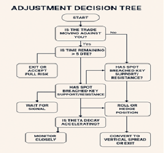
8.7 Adjustment Decision Tree – Flowchart
Key Explanation of Decision Points:
Trade Moving Against You?
- If not, no action is needed.
- If yes, evaluate time and volatility.
Time Remaining > 5 DTE?
- If expiry is near, options lose flexibility.
- If time remains, adjustments are still feasible.
Is IV High?
- High IV allows rolling or converting to spreads for credit.
- Low IV limits premiums — better to cut risk.
Support/Resistance Breached?
- If yes, trend shift is likely. Consider repositioning.
- If no, avoid premature action.
Theta Decay Accelerating?
- If yes, turn long options into spreads or exit.
- If no, observe.
4.1 What are Options Greek?
Options Greeks are essential metrics used to measure the sensitivity of an option’s price to various factors such as changes in the underlying asset price, time, volatility, and interest rates. These metrics provide critical insights for traders to assess risk, make informed decisions, and develop effective trading strategies.
The key Greeks include Delta, which measures the change in an option’s price relative to a ₹1 change in the underlying asset’s price, and Gamma, which indicates the rate at which Delta changes with price movements. Theta measures the impact of time decay on an option’s premium, reflecting how options lose value as expiration nears. Vega assesses an option’s price sensitivity to changes in implied volatility, a critical factor during periods of market uncertainty. Lastly, Rho represents the effect of changes in interest rates on the price of an option.
These Greeks are interconnected, allowing traders to understand how various factors influence options pricing simultaneously. For example, Delta shows price sensitivity, while Gamma monitors changes in Delta. By mastering Options Greeks, traders can effectively manage risk, optimize their portfolio, and capitalize on opportunities in volatile markets. They are indispensable for both novice and experienced traders in navigating the dynamic world of options trading.
4.2 What is Delta (Δ)
Delta (Δ) is one of the most crucial Options Greeks, measuring how sensitive an option’s price is to changes in the price of the underlying asset. It reflects the relationship between the price movement of the underlying asset and the price of the option.
Key Aspects of Delta
For Call Options:
- Delta ranges from 0 to 1.
- A call option with a delta of 0.50 means the option price will increase by ₹0.50 for every ₹1 increase in the price of the underlying asset.
- As the option gets closer to being in-the-money (strike price close to the underlying price), delta approaches 1.
For Put Options:
- Delta ranges from -1 to 0.
- A put option with a delta of -0.50 means the option price will increase by ₹0.50 for every ₹1 decrease in the underlying price.
- As the option becomes deeper in-the-money, delta approaches -1.
Interpreting Delta as Probability:
- Delta can also be seen as the probability of the option expiring in-the-money. For example, a delta of 0.70 for a call option implies a 70% chance of expiring in-the-money.
Delta Behavior
- At-the-Money Options: Delta is approximately 0.50 (for calls) or -0.50 (for puts), meaning they’re equally sensitive to price changes.
- In-the-Money Options: Delta approaches 1 (for calls) or -1 (for puts), reflecting higher sensitivity.
- Out-of-the-Money Options: Delta is closer to 0, as these options are less likely to be exercised.
4.3 Gamma (Γ)
Gamma measures the rate of change in Delta as the underlying asset’s price changes. In other words, Gamma shows how much Delta will increase or decrease when the underlying price moves by ₹1.
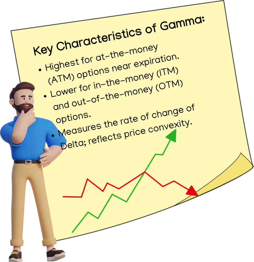
Key Characteristics
- Gamma is largest for at-the-money (ATM) options and near expiration.
- It decreases for in-the-money (ITM) and out-of-the-money (OTM) options.
- Gamma is a second-order derivative of the option’s price with respect to the underlying’s price, reflecting the convexity of the option’s price movement.
Impact of Gamma
- High Gamma indicates that Delta changes rapidly, making the option price highly sensitive to the underlying asset’s movement.
- Low Gamma means that Delta is relatively stable, causing minimal changes in the option’s sensitivity.
Application
Gamma is especially useful in hedging:
- Consider a portfolio with an option whose Delta is 0.5 and Gamma is 0.1. If the underlying price increases by ₹2, Delta will change from 0.5 to 0.7 (0.5 + 0.1 × 2). The trader can use Gamma to adjust their Delta-neutral hedging strategy as the underlying price fluctuates.
Challenges of High Gamma
- High Gamma close to expiration creates significant risks, as small price movements in the underlying can lead to large changes in Delta, requiring constant rebalancing.
4.4 What is Theta (Θ)
Theta measures the impact of time decay on the option’s price, reflecting how much the option’s value decreases each day as it approaches expiration.
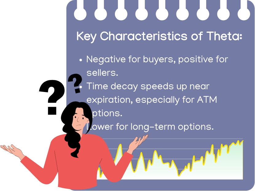
Key Characteristics
- Theta is always negative for option buyers (they lose value over time) and positive for option sellers (they gain value as time passes).
- Time decay accelerates as expiration nears, particularly for at-the-money (ATM) options.
- Long-term options (far from expiration) have lower Theta compared to short-term options.
Impact of Theta
- Time decay works against buyers, as options lose value with each passing day if the underlying price doesn’t move significantly.
- Sellers benefit from Theta as the option premium decreases, especially if the market is range-bound.
Application
For example:
- A call option has a Theta of -5. This means the option will lose ₹5 in value daily, all else being equal.
- Traders selling options (e.g., selling a straddle or covered call) rely on Theta to profit from time decay when they expect minimal price movement.
Theta Management
Buyers must choose their timing carefully, as purchasing options with high Theta can lead to substantial losses if the expected price movement doesn’t occur before expiration.
4.5 Vega (ν)
Vega measures the sensitivity of an option’s price to changes in implied volatility (IV). It shows how much the option’s price will increase or decrease for a 1% change in IV.
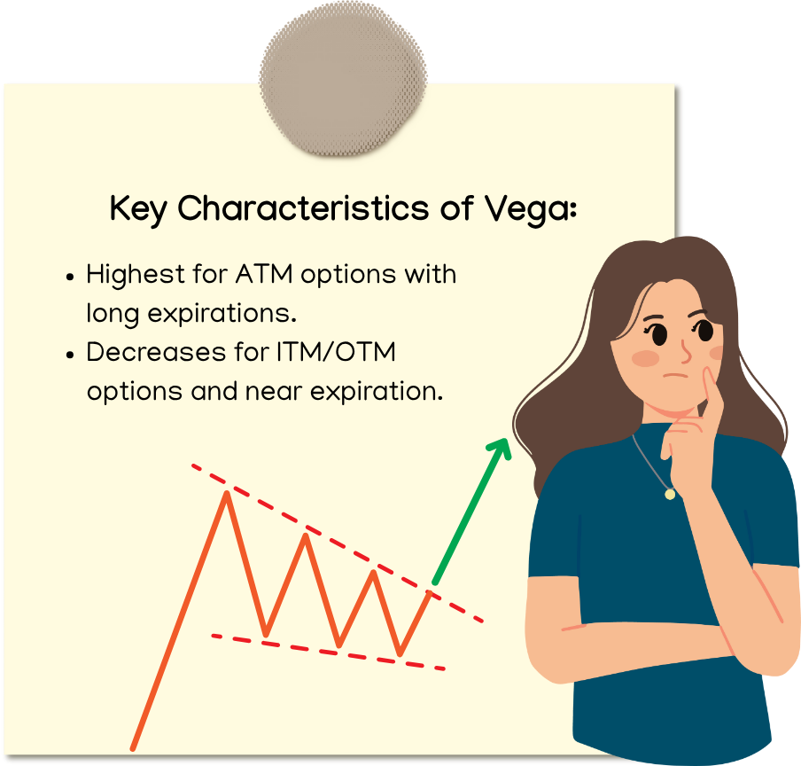
Key Characteristics
- Vega is highest for at-the-money (ATM) options with longer expiration periods.
- It decreases for in-the-money (ITM) or out-of-the-money (OTM) options and as expiration approaches.
Impact of Vega
- When implied volatility rises, option prices (both calls and puts) increase, benefiting buyers.
- When implied volatility drops, option prices decrease, benefiting sellers due to the volatility “crush.”
Application
Suppose an option has a Vega of 0.10 and its premium is ₹100. If implied volatility rises by 5%, the option’s price increases by ₹0.10 × 5 = ₹0.50, making the new premium ₹100.50.
Volatility Strategies
- Buyers look for opportunities in high-volatility environments, expecting significant price movements.
- Sellers capitalize on low volatility or post-event scenarios (volatility crush) to profit from declining premiums.
4.6 Rho (ρ)
Rho measures the sensitivity of an option’s price to changes in the risk-free interest rate. It is less influential compared to other Greeks but becomes significant for long-term options.
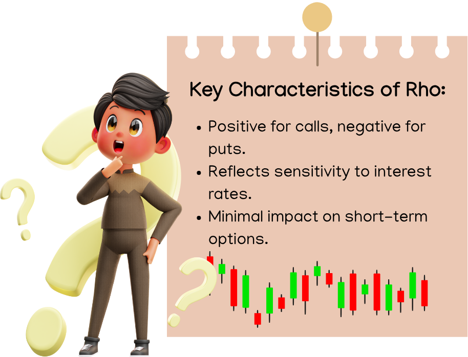
Key Characteristics
- Call Options: Rho is positive because higher interest rates reduce the present value of the strike price, making calls more attractive.
- Put Options: Rho is negative because higher interest rates reduce the present value of the strike price, making puts less attractive.
- Rho’s impact is minimal for short-term options, as interest rate changes affect them less.
Impact of Rho
- A long-term call option with a Rho of 0.05 will gain ₹0.05 in value for every 1% increase in interest rates.
- A long-term put option with a Rho of -0.05 will lose ₹0.05 in value for every 1% increase in interest rates.
Application
Rho is important for traders focusing on longer-duration options or during periods of fluctuating interest rates, such as central bank policy announcements.
How the Greeks Work Together
- Gamma supports Delta: It refines Delta’s effectiveness by predicting its changes.
- Theta interacts with Vega: In high-volatility scenarios, Vega can offset Theta’s time decay.
- Rho complements the others: It factors in macroeconomic changes, particularly for long-term options.
4.7 Interplay of Greeks

The interplay of Greeks is critical in options trading as each Greek captures a specific risk factor. Monitoring and combining them provides a holistic view of how options behave under different scenarios. Let’s break down the points you mentioned in detail:
- Gamma Adjusts Delta
What It Means:
- Delta measures how much the option’s price will change with a ₹1 change in the underlying asset price.
- Gamma measures the rate of change of Delta for every ₹1 change in the underlying price. Essentially, Gamma adjusts Delta dynamically as the underlying price moves.
Why It Matters:
- Delta doesn’t remain constant; it changes as the price of the underlying asset fluctuates.
- High Gamma indicates that Delta changes rapidly, making the option more sensitive to price movements.
- Low Gamma means that Delta changes slowly, offering stability.
Practical Implications:
- Hedging:
- A Delta-neutral portfolio (where Delta = 0) must be adjusted frequently if Gamma is high. For example, as the underlying asset moves, traders rebalance their positions to keep Delta neutral.
- Gamma hedging ensures that adjustments account for the rapid changes in Delta.
Example:
- A call option has Delta of 0.50 and Gamma of 0.10. If the underlying price rises by ₹2, Delta increases to 0.70 (0.50 + 0.10 × 2). The trader must adjust their position to maintain Delta neutrality.
- Vega Offsets Theta During Volatile Conditions
What It Means:
- Theta measures the impact of time decay on an option’s price. As time passes, an option loses value due to Theta, especially for buyers.
- Vega measures the sensitivity of an option’s price to changes in implied volatility (IV). When volatility rises, Vega increases the option premium.
Why It Matters:
- During periods of high volatility, the increase in Vega can offset the loss caused by Theta. This is particularly beneficial for buyers of options.
- In contrast, when volatility drops, Vega decreases the option premium, amplifying the losses caused by Theta. This situation benefits sellers, as they profit from both time decay and volatility reduction.
Practical Implications:
- Volatility-Based Strategies:
- If a trader expects high volatility (e.g., before earnings reports), they might buy options to benefit from Vega outweighing Theta.
- If volatility crush is expected (e.g., after an event), sellers profit as both Vega and Theta work in their favor.
Example:
- A trader buys an at-the-money option with Theta of -2 and Vega of 0.10. If volatility increases by 5%, the option gains ₹0.50 due to Vega (0.10 × 5), potentially offsetting the ₹2 loss from Theta decay.
- Rho Complements Long-Term Interest Rate Strategies
What It Means:
- Rho measures the sensitivity of an option’s price to changes in interest rates.
- Changes in interest rates primarily affect the present value of the strike price. Call options gain value as interest rates rise, while put options lose value.
Why It Matters:
- Rho becomes significant for long-term options or during periods of interest rate fluctuations.
- It helps traders assess the broader macroeconomic impact on their positions, especially when central banks adjust interest rates.
Practical Implications:
- Long-Term Hedging:
- For long-term options (e.g., LEAPS), traders consider Rho to understand how rate changes will impact their portfolio value.
- Traders holding long-dated call options benefit from rising interest rates due to positive Rho.
Example:
- A trader holds a call option with a Rho of 0.05. If interest rates increase by 1%, the option’s price rises by ₹0.05. For portfolios sensitive to interest rates, Rho becomes a critical factor.
|
Greek |
Most Affected Strategies |
Importance |
|
Delta |
Covered Calls, Long Calls |
Directional Bias |
|
Gamma |
Gamma Scalping, Short Straddles |
Adjustments, Volatility Risk |
|
Theta |
Iron Condor, Credit Spreads |
Time Decay Income |
|
Vega |
Long Straddles, Calendar Spreads |
Volatility Trading |
|
Rho |
LEAPS, Long-Term Hedging |
Interest Rate Risk |
4.8 When is Greek most important?

|
Greek |
When is it Important? |
Strategies Most Sensitive |
|
Delta |
Directional price moves |
Long Calls/Puts, Spreads, Covered Calls |
|
Gamma |
Rapid price changes, hedging |
Straddles, ATM near expiry, Delta-neutral |
|
Theta |
Time decay near expiry |
Short Options, Credit Spreads, Iron Condors |
|
Vega |
Volatility changes |
Long Straddles, Calendars, Long Options |
|
Rho |
Interest rate shifts |
LEAPS, Bond Options, Long-term Calls/Puts |
4.9 Risk Graphs

Delta
Delta risk graphs are used to assess and manage option trading risks. Here’s why they are important:
- Risk Management:Traders use delta to understand how an option’s price will react to movements in the underlying asset. A high delta means the option moves almost like the stock itself, while a low delta means less sensitivity.
- Hedging Strategies:Institutions and traders use delta to hedge portfolios against market movements. A delta-neutral strategy, for example, balances positive and negative deltas to reduce risk exposure.
- Predicting Option Behavior:Seeing how delta shifts helps traders anticipate how an option will behave as the stock price moves and decide whether to buy or sell options.
- Position Adjustment:A changing delta can signal when to adjust positions to maintain a desired level of exposure or protection.
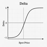
This graph represents the relationship between delta and the underlying asset’s spot price. Here’s how to interpret it:
- Delta (Y-Axis):Measures how much an option’s price changes with a ₹1 movement in the underlying asset. For call options, delta ranges from 0 to 1, and for put options, it ranges from 0 to -1.
- Spot Price (X-Axis):Represents the market price of the underlying asset.
- Shape of the Curve:
- For call options, delta increases as the spot price rises, moving closer to 1.
- For put options, delta decreases as the spot price rises, moving closer to -1.
Gamma Effect:This influences how steeply delta changes. A high gamma means delta adjusts rapidly when the spot price is near the strike price.
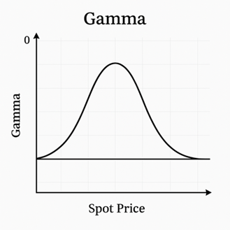
Gamma peaks at ATM and drops for ITM/OTM
This graph illustrates the behavior of gamma in relation to the underlying asset’s price and the option’s moneyness (ITM, ATM, OTM). Here’s how it works:
- Gamma (Y-Axis):Measures the rate of change of delta as the underlying asset price changes. A higher gamma means delta adjusts rapidly.
- Spot Price (X-Axis):Represents the market price of the underlying asset.
- Peak at ATM:Gamma is highest for at-the-money (ATM) options because delta is most sensitive when the option is near its strike price.
- Drop for ITM and OTM:Gamma declines as options move in-the-money (ITM) or out-of-the-money (OTM) because delta stabilizes.
- ITM options:Already have significant intrinsic value, so delta remains high and changes slowly.
- OTM options:Have low delta and are less sensitive to price movements.
Essentially, gamma is crucial for options traders because it affects how aggressively delta moves, helping them anticipate price shifts and adjust their strategies accordingly.
Theta decay over time (exponential curve)
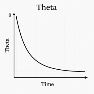
Theta measures how the value of an option decreases as time passes, especially as expiration approaches. The decay tends to follow an exponential curve, meaning that early in an option’s life, the time decay is gradual. However, as expiration nears, theta accelerates rapidly, causing the option’s value to drop significantly.
Key takeaways:
- Time Factor:Options lose value over time, assuming other factors remain constant.
- Acceleration Near Expiry:The decay rate speeds up as the option gets closer to expiration.
- Impact on Trading:Traders managing short options must be mindful of theta decay, while long option holders often struggle with time working against them.
Vega highest at ATM, especially for long-dated options
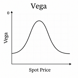
Vega measures an option’s sensitivity to changes in implied volatility. It is highest for at-the-money (ATM) options because volatility has the greatest impact when the option is near the strike price. The effect is even more pronounced for long-dated options, as they have more time for implied volatility to influence their price.
Key points:
- ATM Options: Experience the strongest Vega effects since small volatility shifts significantly impact the option’s value.
- Long-Dated Options: Higher Vega because time amplifies the role of volatility.
- Short-Term vs. Long-Term: Short-term options have lower Vega since they have less time for volatility to play a role.
4.10 Real World Examples

1. Delta (Δ) – Directional Sensitivity
When is it most important?
Delta measures how much an option’s price is expected to change for a ₹1 change in the underlying asset’s price. It is crucial when you have a directional view on the market and want to understand how option premiums will respond to price movements.
Strategies most sensitive to Delta:
- Long Calls and Puts
- Covered Calls
- Protective Puts
- Vertical Spreads
📌 Example:
Suppose you own 100 shares of Infosys, currently trading at ₹1,500. You decide to sell a call option with a strike price of ₹1,550, expiring in one month, for a premium of ₹30. This call option has a Delta of 0.55.
If Infosys’s stock price rises by ₹10 to ₹1,510, the price of the call option is expected to increase by ₹5.50 (₹10 × 0.55). This means the option you sold becomes more valuable, potentially leading to a loss if you need to buy it back. Understanding Delta helps you assess how much the option’s price will move relative to the stock’s price, aiding in strike price selection and risk management.
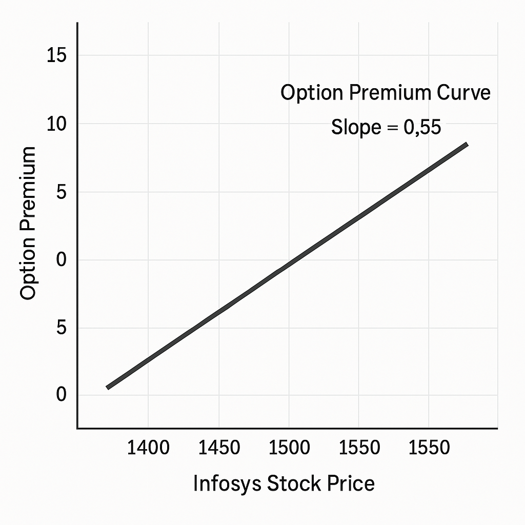
📊 Graph Description:
- X-axis: Infosys Stock Price
- Y-axis: Option Premium Curve:
- A straight line with a slope of 0.55, indicating that for every ₹1 increase in stock price, the option premium increases by ₹0.55 give image
2. Gamma (Γ) – Rate of Change of Delta
When is it most important?
Gamma measures the rate of change of Delta with respect to the underlying asset’s price. It is most significant for at-the-money options nearing expiration, as small movements in the underlying can lead to large changes in Delta.
Strategies most sensitive to Gamma:
- Long Straddles and Strangles
- Short-term ATM Options
- Delta-Neutral Portfolios
📌 Example:
Imagine you’re trading NIFTY options, and the index is at 18,000. You purchase a 18,000 strike price call option expiring in two days, which has a Delta of 0.50 and a Gamma of 0.10.
If NIFTY moves up by 100 points to 18,100, the Delta of your option would increase by 0.10 to 0.60. This means the option’s sensitivity to further price movements has increased, and its price will now change more rapidly with NIFTY’s movements. Gamma helps you understand how your position’s risk profile evolves with market movements, especially near expiration.
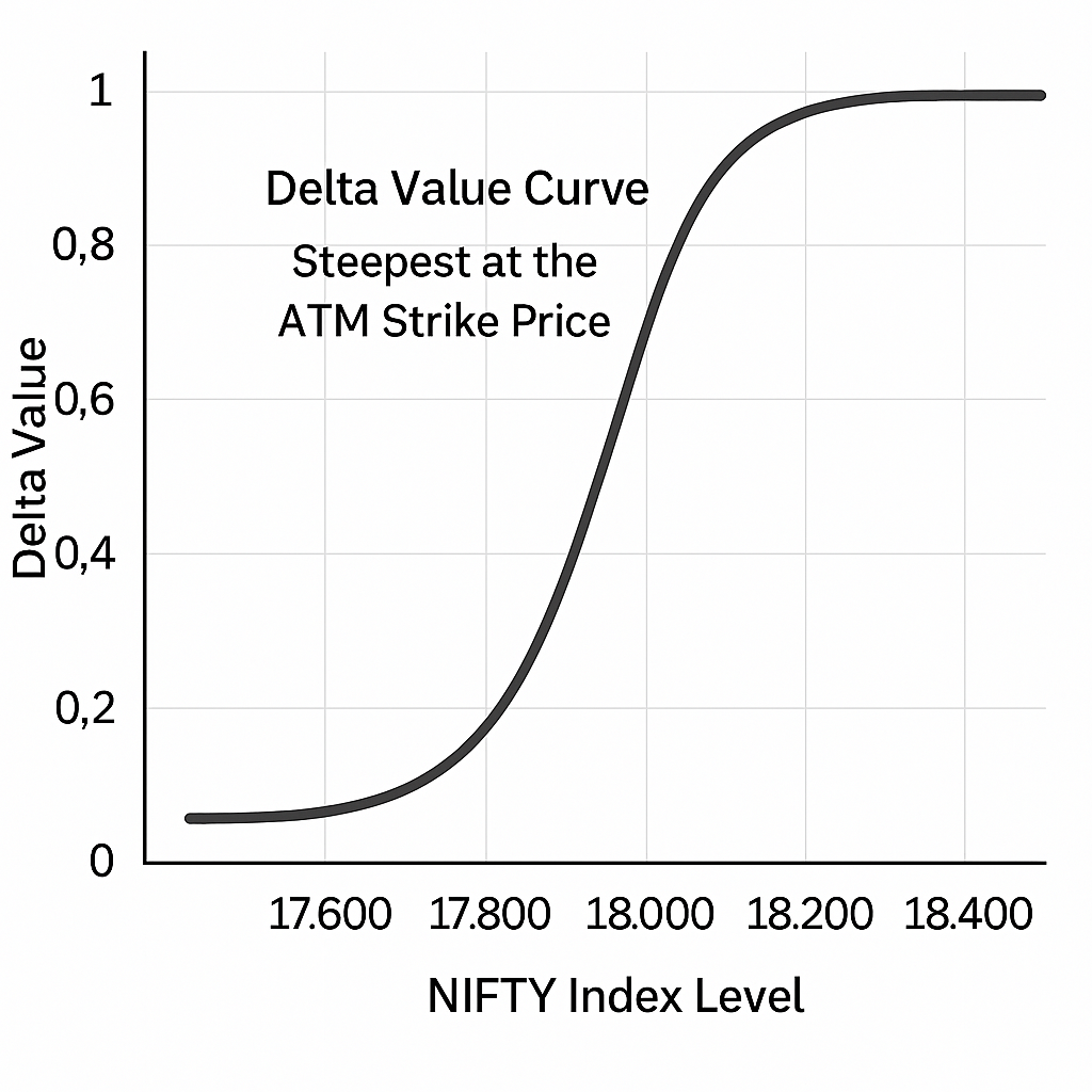
📊 Graph Description:
- X-axis: NIFTY Index Level
- Y-axis: Delta Value
- Curve: An S-shaped curve that is steepest at the ATM strike price, illustrating how Delta changes more rapidly near the ATM as expiration approaches.
-
Theta (Θ) – Time Decay
When is it most important?
Theta measures the rate at which an option’s value decreases as it approaches expiration, assuming all other factors remain constant. It is particularly important for options sellers and for short-term trading strategies.
Strategies most sensitive to Theta:
- Short Options (Naked Calls/Puts)
- Credit Spreads
- Iron Condors
- Calendar Spreads (Short Leg)
📌Example:
Suppose you sell a Bank Nifty 40,000 strike price call option expiring in three days for a premium of ₹100. The option has a Theta of -₹20.
This means that, all else being equal, the option’s premium will decrease by ₹20 each day due to time decay. If Bank Nifty remains below 40,000, you can potentially profit from the erosion of the option’s value over time. Theta is crucial for understanding how the passage of time affects option premiums, especially for short-term strategies.
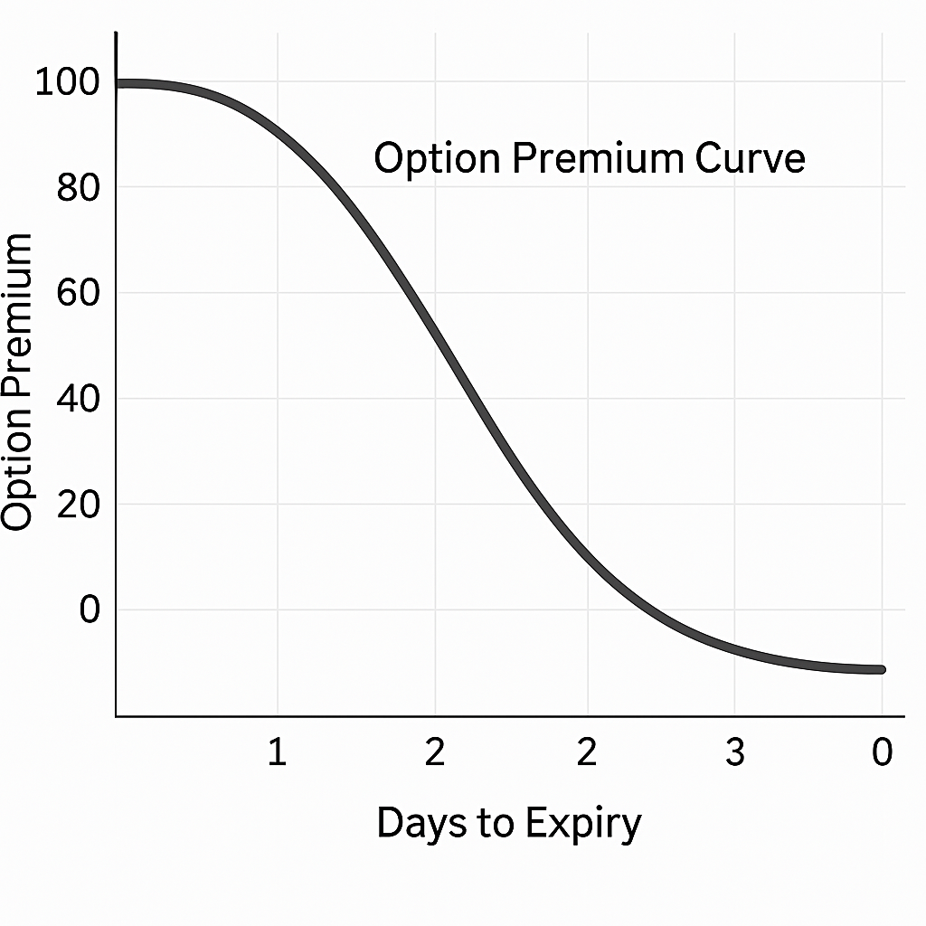
📊 Graph Description:
- X-axis: Days to Expiry
- Y-axis: Option Premium
- Curve: A downward-sloping curve that becomes steeper as expiration approaches, indicating accelerated time decay. give image
Vega (ν) – Volatility Sensitivity
When is it most important?
Vega measures the sensitivity of an option’s price to changes in the implied volatility of the underlying asset. It is vital when trading strategies that are sensitive to volatility changes, such as during earnings announcements or major economic events.
Strategies most sensitive to Vega:
- Long Straddles and Strangles
- Long Options
- Calendar and Diagonal Spreads
📌 Example:
Consider you anticipate increased volatility in Reliance Industries due to an upcoming earnings report. You buy a straddle by purchasing both a call and a put option at the ₹2,500 strike price, each with a Vega of ₹0.15.
If implied volatility increases by 5% after the earnings announcement, each option’s premium is expected to increase by ₹0.75 (₹0.15 × 5), benefiting your position. Vega helps you assess how changes in market expectations of volatility can impact your options’ value.
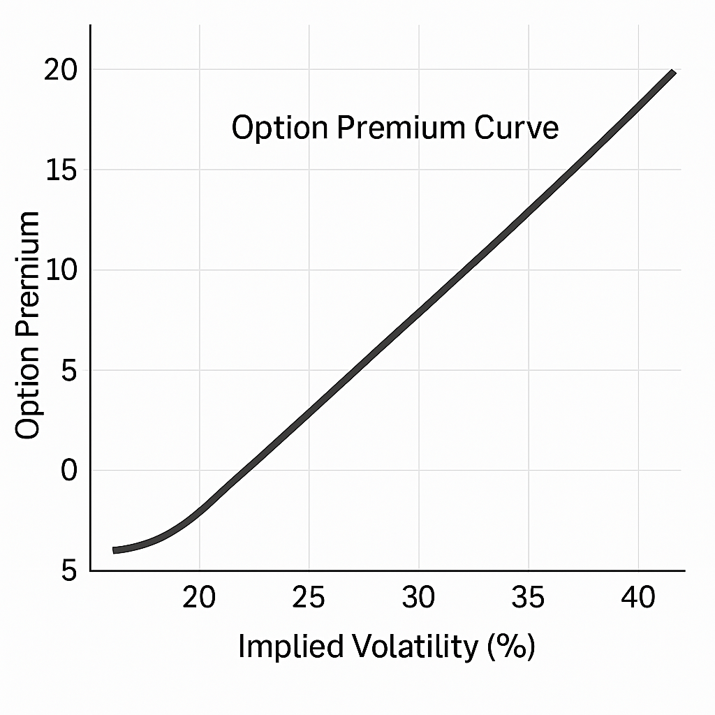
📊 Graph Description:
- X-axis: Implied Volatility (%)
- Y-axis: Option Premium
- Curve: An upward-sloping line, showing that as implied volatility increases, the option premium increases proportionally
Rho (ρ) – Interest Rate Sensitivity
When is it most important?
Rho measures the sensitivity of an option’s price to changes in the risk-free interest rate. It becomes more relevant for long-term options and in environments where interest rates are changing significantly.
Strategies most sensitive to Rho:
- Long-term Options (LEAPS)
- Interest Rate Sensitive Instruments
- Bond Options
📌 Example:
Suppose you hold a long-term call option on HDFC Bank with a strike price of ₹1,500, expiring in one year, and a Rho of 0.05.
If the Reserve Bank of India increases interest rates by 1%, the value of your call option is expected to increase by ₹0.05 (₹1 × 0.05), assuming all other factors remain constant. While Rho is often less significant than other Greeks, it can impact the pricing of long-dated options in changing interest rate environments.
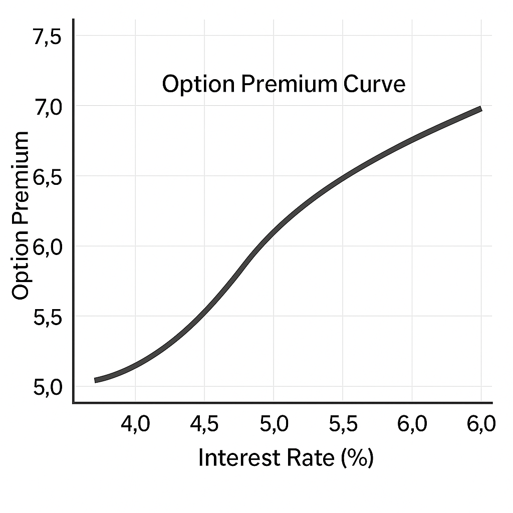
Graph Description:
- X-axis: Interest Rate (%)
- Y-axis: Option Premium
- Curve: A gently upward-sloping line, indicating that as interest rates increase, the premium of call options increases slightly.
Summary Table:
|
Greek |
Significance |
Sensitive Strategies |
Indian Market Example |
|
Delta (Δ) |
Measures option price change relative to underlying asset price changes |
Long Calls/Puts, Covered Calls, Vertical Spreads |
Infosys Covered Call |
|
Gamma (Γ) |
Measures rate of change of Delta; important for ATM options near expiration |
Straddles, Short-term ATM Options, Delta-Neutral Portfolios |
NIFTY ATM Call Option |
|
Theta (Θ) |
Measures time decay; crucial for options sellers |
Short Options, Credit Spreads, Iron Condors |
Bank Nifty Short Call |
|
Vega (ν) |
Measures sensitivity to volatility changes; important during events |
Long Straddles/Strangles, Calendar Spreads |
Reliance Earnings Straddle |
|
Rho (ρ) |
Measures sensitivity to interest rate changes; relevant for long-term options |
LEAPS, Bond Options |
HDFC Bank Long-Term Call |
4.11 Greeks in Multi-Leg Strategies

Offsetting Greeks in Spreads
Calendar Spreads (Vega and Theta):
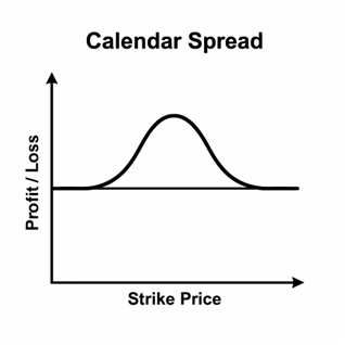
- Structure:Involves selling a near-term option and buying a longer-term option at the same strike price.
- Greek Dynamics:
- Vega:The long-term option has higher Vega, making the position sensitive to changes in implied volatility.
- Theta:The near-term option decays faster, benefiting the seller due to higher Theta.
Practical Insight:If implied volatility increases, the long-term option’s value rises more than the short-term option’s loss, leading to a net gain.
Iron Condors (Delta and Gamma):
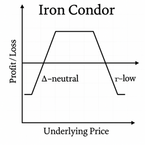
- Structure:Combines a bear call spread and a bull put spread, aiming to profit from low volatility.
- Greek Dynamics:
- Delta:Designed to be Delta-neutral, minimizing directional risk.
- Gamma:Low Gamma implies the position is less sensitive to large price movements.
Practical Insight:Ideal in stable markets, but sudden price swings can lead to significant losses due to Gamma risk.
Balancing Risk in Neutral Strategies
Straddles and Strangles:
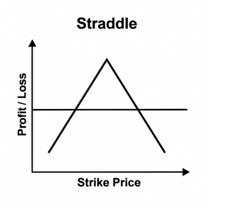
- Structure:Involves buying or selling both call and put options at the same (straddle) or different (strangle) strike prices.
- Greek Dynamics:
- Delta:Neutral at initiation but can become directional with price movements.
- Gamma:High Gamma near expiration, leading to rapid Delta changes.
- Theta:Short positions benefit from time decay; long positions suffer.
Practical Insight:Short straddles/strangles can be profitable in low volatility but carry significant risk if the underlying moves sharply.
Adjusting Across Expirations
Diagonal Spreads:
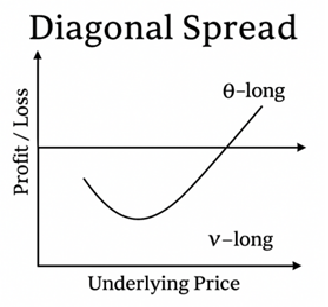
- Structure:Combines options of different strike prices and expiration dates.
- Greek Dynamics:
- Theta:Short-term option decays faster, benefiting the position.
- Vega:Long-term option is more sensitive to volatility changes.
Practical Insight:Useful when expecting gradual price movement and an increase in volatility.
4.12 Greeks in Expiry Trading (Weekly Options)

Theta and Gamma Risks Near Expiry
- Theta:Time decay accelerates as expiration approaches, especially for at-the-money (ATM) options.
- Gamma:Becomes more pronounced near expiry, causing Delta to change rapidly with small price movements.
- Practical Insight:Shorting ATM options close to expiry can be lucrative due to high Theta but risky due to Gamma spikes.
Gamma Spikes and Short Straddles
- Scenario:On expiry day, a short straddle (selling both call and put at the same strike) can be profitable if the underlying remains stable.
- Risk:A sudden price move can lead to significant losses due to rapid Delta changes driven by high Gamma.
- Practical Insight:Implementing stop-loss orders and closely monitoring positions is crucial on expiry days.
Delta Hedging Challenges
- Issue:Near expiry, high Gamma makes Delta hedging difficult, as small price changes require frequent adjustments.
- Practical Insight:Traders should be cautious with Delta-neutral strategies close to expiration and consider reducing position sizes.
4.13 Practical Tips for Retail Traders

- Avoid Shorting ATM Options on Thursdays:High Gamma risk can lead to significant losses with minimal price movement.
- Be Wary of Long Straddles Without Volatility Increase:If implied volatility doesn’t rise as expected, Theta decay can erode profits.
- Delta-Neutral Isn’t Risk-Neutral:Even if Delta is neutralized, Gamma and Vega can introduce significant risks.
- Monitor Implied Volatility:Understanding Vega’s impact is crucial, especially when trading around events like earnings announcements.
- Use Stop-Loss Orders:Protect against unexpected market movements, especially near expiry.
- Educate Yourself Continuously:Options trading is complex; ongoing learning is essential for success.